Laplace Transform Calculator
Laplace Transform
Enter a function of t (e.g., "sin(a*t)", "exp(-t)", "t**2"):

Inverse Laplace Transform
Enter a function of s (e.g., "1/(s**2+1)", "s/(s**2+a**2)"):
About Laplace Transforms
Laplace transforms, named after the renowned French mathematician Pierre-Simon Laplace (1749-1827), are a powerful mathematical tool widely used in various fields of science and engineering. These integral transforms provide a method to convert complex differential equations into simpler algebraic equations, making them easier to solve and analyze.
Historical Context
The concept of Laplace transforms emerged from Laplace's work on probability theory and celestial mechanics in the late 18th and early 19th centuries. However, it wasn't until the 20th century that their full potential in solving differential equations and analyzing systems was realized. The advent of operational calculus, developed by Oliver Heaviside, brought Laplace transforms into the spotlight, particularly in the fields of physics and engineering.
Mathematical Definition
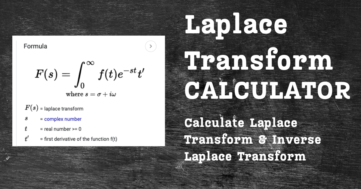
Formally, the Laplace transform of a function f(t), defined for all real numbers t ≥ 0, is the function F(s) defined by:
F(s) = ℒ{f(t)} = ∫0∞ e-st f(t) dt
Here, s is a complex number frequency parameter. This integral transform essentially converts a function of time (t) into a function of complex frequency (s). The inverse Laplace transform reverses this process, allowing us to return from the frequency domain to the time domain.
Applications in Science and Engineering
Laplace transforms have found extensive applications across various disciplines:
- Control Systems Engineering: They are fundamental in analyzing the stability and transient response of control systems. Transfer functions, a cornerstone of control theory, are often expressed in terms of Laplace transforms.
- Electrical Engineering: Circuit analysis becomes more manageable in the Laplace domain, especially for complex circuits with multiple components. They're also crucial in signal processing and communications systems.
- Mechanical Engineering: Vibration analysis, heat transfer problems, and fluid dynamics often employ Laplace transforms to simplify complex differential equations.
- Physics: They're used in solving wave equations, quantum mechanics problems, and in the analysis of linear time-invariant systems.
- Mathematics: Beyond their practical applications, Laplace transforms are studied in their own right in complex analysis and operator theory.
Key Properties and Advantages
Several properties make Laplace transforms particularly useful:
- Linearity: The transform of a sum is the sum of the transforms, allowing complex problems to be broken down into simpler parts.
- Differentiation and Integration: These operations in the time domain correspond to simple algebraic operations in the Laplace domain, often simplifying the solution process.
- Convolution: The convolution of functions in the time domain becomes a simple multiplication in the Laplace domain.
- Initial Value Problems: Laplace transforms are especially adept at handling initial value problems in differential equations.
Modern Computational Approaches
While the theory of Laplace transforms is well-established, modern computational tools have greatly enhanced their practical application. Our calculator, for instance, utilizes SymPy, a powerful symbolic mathematics library for Python. This allows for quick and accurate calculations of Laplace transforms and their inverses, as well as step-by-step solutions to complex problems.
The use of computational tools like SymPy has opened up new possibilities in education and research. Students can now easily visualize and experiment with Laplace transforms, while researchers can tackle more complex problems that were previously intractable through manual calculations alone.
Conclusion
Laplace transforms remain a crucial tool in many fields of science and engineering. Their ability to simplify complex problems, especially in the analysis of linear systems, ensures their continued relevance in both academic and practical contexts. As computational tools continue to evolve, we can expect even more innovative applications of Laplace transforms in solving real-world problems.
For those interested in delving deeper into the mathematics and applications of Laplace transforms, we recommend exploring academic resources and advanced textbooks. The Wikipedia page on Laplace transforms also provides a comprehensive overview and can serve as a starting point for further research.
Theory of Laplace Transforms
Definition
The Laplace transform of a function f(t), defined for all real numbers t ≥ 0, is the function F(s), defined by:
F(s) = ℒ{f(t)} = ∫0∞ e-st f(t) dt
where s is a complex number frequency parameter.
Properties
- Linearity: ℒ{af(t) + bg(t)} = aℒ{f(t)} + bℒ{g(t)}
- Differentiation: ℒ{f'(t)} = sF(s) - f(0)
- Integration: ℒ{∫0t f(τ)dτ} = (1/s)F(s)
- Time shift: ℒ{f(t-a)u(t-a)} = e-asF(s)
- Frequency shift: ℒ{eatf(t)} = F(s-a)
- Convolution: ℒ{f(t) * g(t)} = F(s)G(s)
Common Laplace Transform Pairs
| f(t) | F(s) = ℒ{f(t)} |
|---|---|
| 1 (unit step) | 1/s |
| t | 1/s2 |
| eat | 1/(s-a) |
| sin(ωt) | ω/(s2 + ω2) |
| cos(ωt) | s/(s2 + ω2) |
Examples
Example 1: Laplace transform of eat
Let's find the Laplace transform of f(t) = eat:
F(s) = ∫0∞ e-st eat dt
= ∫0∞ e(a-s)t dt
= [-1/(a-s) e(a-s)t]0∞
= 0 - [-1/(a-s)] = 1/(s-a)
Therefore, ℒ{eat} = 1/(s-a)
Example 2: Solving a differential equation
Let's solve the differential equation: y'' + 4y = 0, y(0) = 1, y'(0) = 0
- Take the Laplace transform of both sides:
ℒ{y''} + 4ℒ{y} = 0
- Use the differentiation property:
(s2Y(s) - sy(0) - y'(0)) + 4Y(s) = 0
- Substitute initial conditions:
(s2Y(s) - s) + 4Y(s) = 0
- Solve for Y(s):
(s2 + 4)Y(s) = s
Y(s) = s / (s2 + 4)
- Recognize this as the Laplace transform of cos(2t):
y(t) = cos(2t)
Thus, the solution to the differential equation is y(t) = cos(2t).
Frequently Asked Questions
What is a Laplace transform?
A Laplace transform is an integral transform that converts a function of a real variable t (often time) to a function of a complex variable s (frequency). It's widely used in mathematics, physics, and engineering to solve differential equations and analyze linear time-invariant systems.
How do I use this Laplace transform calculator?
To use the calculator, enter a function of t in the input field for Laplace transform (e.g., 'sin(a*t)', 'exp(-t)', 't**2'). Click 'Calculate Laplace Transform' to get the result. For inverse transforms, enter a function of s in the inverse input field and click 'Calculate Inverse Laplace Transform'.
What types of functions can I input?
You can input a wide range of functions, including trigonometric functions (sin, cos), exponentials (exp), polynomials, and combinations of these. The calculator uses SymPy, so it can handle most common mathematical functions and expressions.
Is this calculator free to use?
Yes, this Laplace transform calculator is completely free to use. There are no hidden charges or subscription fees.
How accurate are the results?
The calculator uses SymPy, a symbolic mathematics library for Python, which provides highly accurate results. However, for very complex functions or special cases, it's always a good idea to verify the results with other methods or consult with a mathematics professional.